Detecting Credit Card Fraud

Introduction

A popular imbalanced Kaggle dataset contains credit card transactions from September 2013. Transactions occurred over two days, and there are 492 fraudulent transactions out of 284,807 total (thus fraudulent transactions account for just 0.172% of all transactions). I found a number of submissions on Kaggle fell short of the kind of thorough investigation and modeling that might convince a financial firm to use the model in production. After observing a number of submissions, the most common errors I found were:

1. Using accuracy alone to measure performance: Always guessing that a transaction is NOT fraudulent results in an accuracy of 99.8%, which also improves as more users make non-fraudulent transactions. This is a misguided performance metric that is disingenous to use. I use F1 score to make my process easy to compare with others on Kaggle, but at the end I propose a smarter way to think about the true cost of a false negative (not flagging fraud) vs. a false positive (freezing a user's credit card due to a normal transaction).

2. Oversampling and/or scaling before the train/test split. This form of data leakage invalidates any results on a holdout test set. This is by far the most common error I found for those claiming F1 scores above 0.90.

3. No insight into model behavior. This isn’t a significant error as far as Kaggle competitions are concerned, but stakeholders (especially for financial firms) are unlikely to accept a model that basically does a bit of preprocessing and then puts everything into a black-box-esque algorithm. At least some visibility, even in the form of data visualizations for non-linear methods, is key to get stakeholder buy in.

So let's get into how I'd go about analyzing this dataset. The very first thing is to split it 70:30 into a training set and test set. Because the dataset is highly imbalanced, to ensure the training and test sets are representative we need to be careful to use stratified random sampling so that the distribution of classes in each sample matches the overall population.

Exploratory Data Analysis (EDA)

We’re told that Features V1, V2, … V28 are the principal components obtained with PCA. That means we should first investigate Time and Amount, which are not transformed. For simplicity, Time (in seconds) can be adjusted to Hours. Amount is severely right skewed, so we'll use a log-transform to make the distribution more normal and easier to interpret.

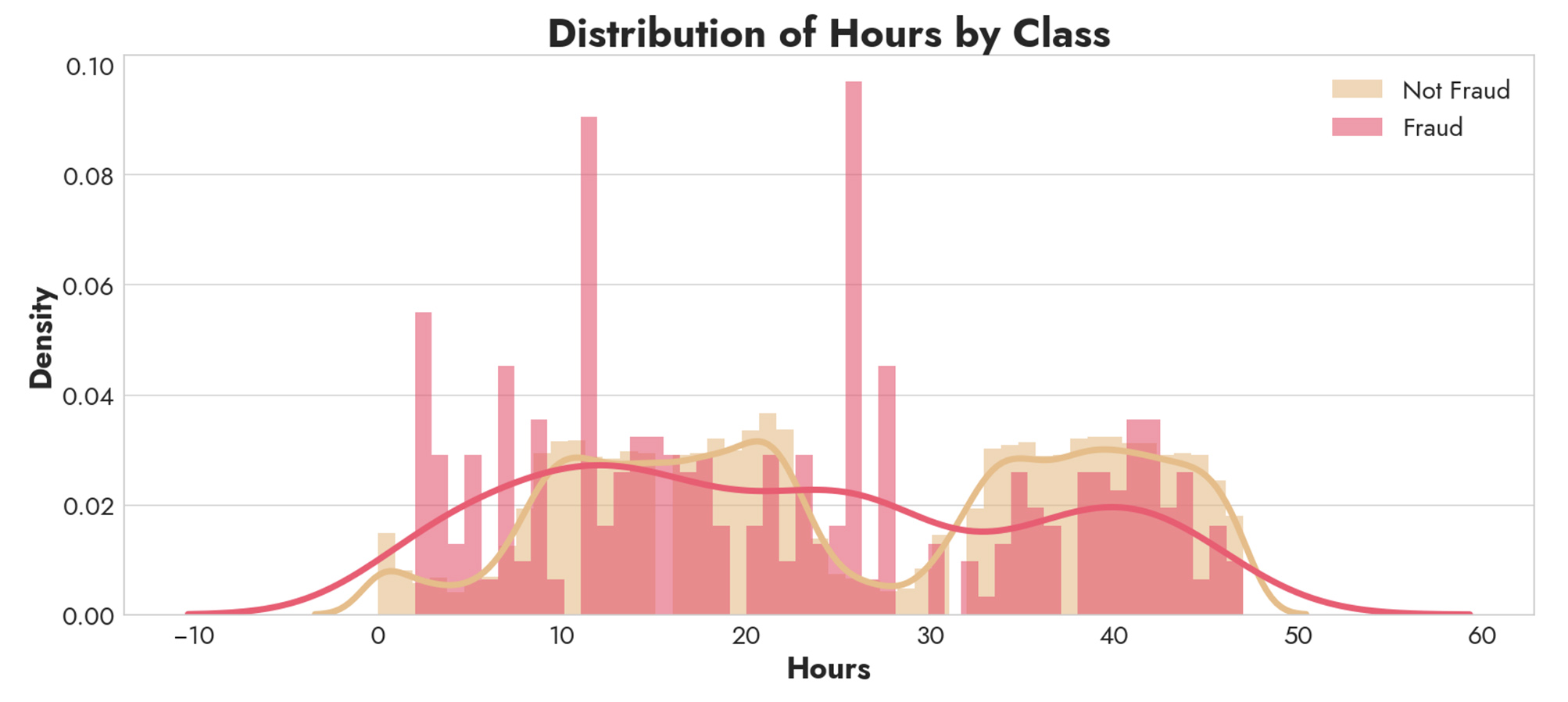
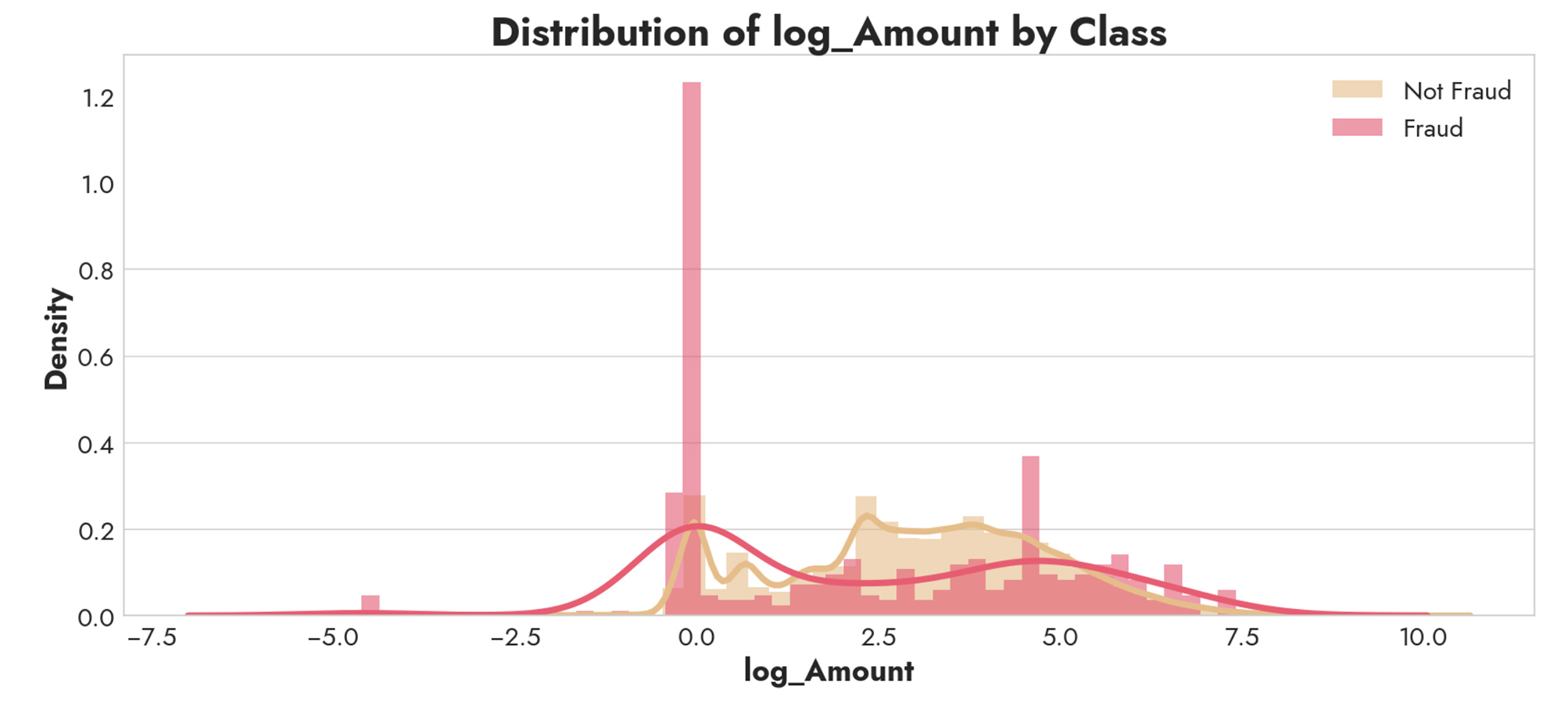
The rate of fraudulent transactions is 5.5x higher (0.94% vs. 0.17%) when the transaction amount is $0.00, which is interesting. However, log_Amount does not separate the two classes into two distinct distributions, so we should keep looking. Hours is more promising. Whereas normal transactions are bimodal (perhaps between morning and evening) fraudulent transactions happen more often at abnormal hours of the day. So Hours could be a good feature for us to include.

Feature Selection

This still leaves us with 28 other features (V1 - V28), which is quite a bit. We'd like some form of feature selection to whittle down to the most predictive features. One method we could use is sklearn’s SelectKBest feature selection function. This is a quick and easy way to check how extreme values are using a chi-squared distribution, which is desirable to find which features contain anomalous values that can be used to distinguish fraud. Running a simple SelectKBest with k=10, we get V3, V4, V7, V10-V12, V14, V16-V18 as the best features. We’ll use a z-score scaling (standardization) on all our features, and then visualize these distributions along with Hours from above.

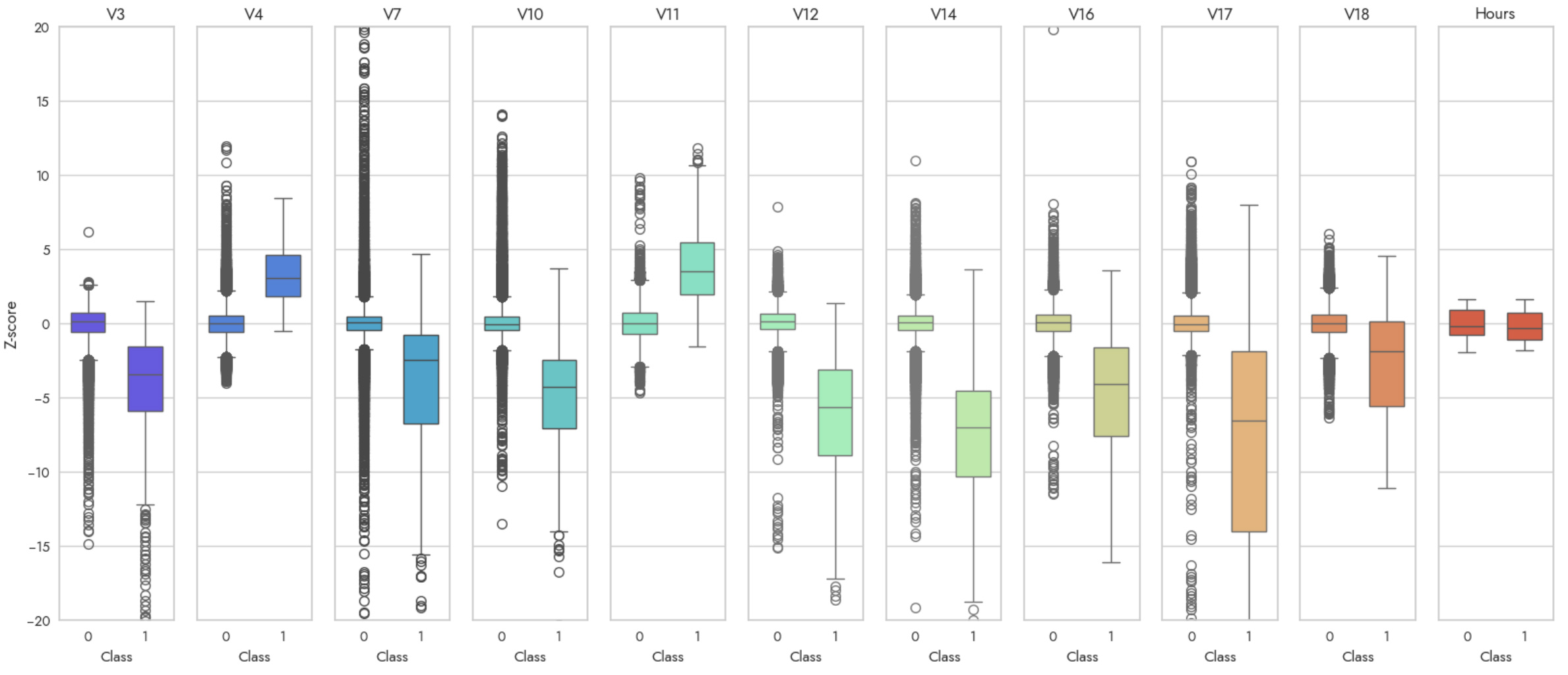
Although this is a quicker way to achieve something similar to the histograms we were using above, notice that some features (like Hours) which may have biomodal distributions are obscured and the distributions between classes don't look that distinct. That's why these methods are complementary, not substitutes for each other. Finally, we can check all the remaining features just for completeness.

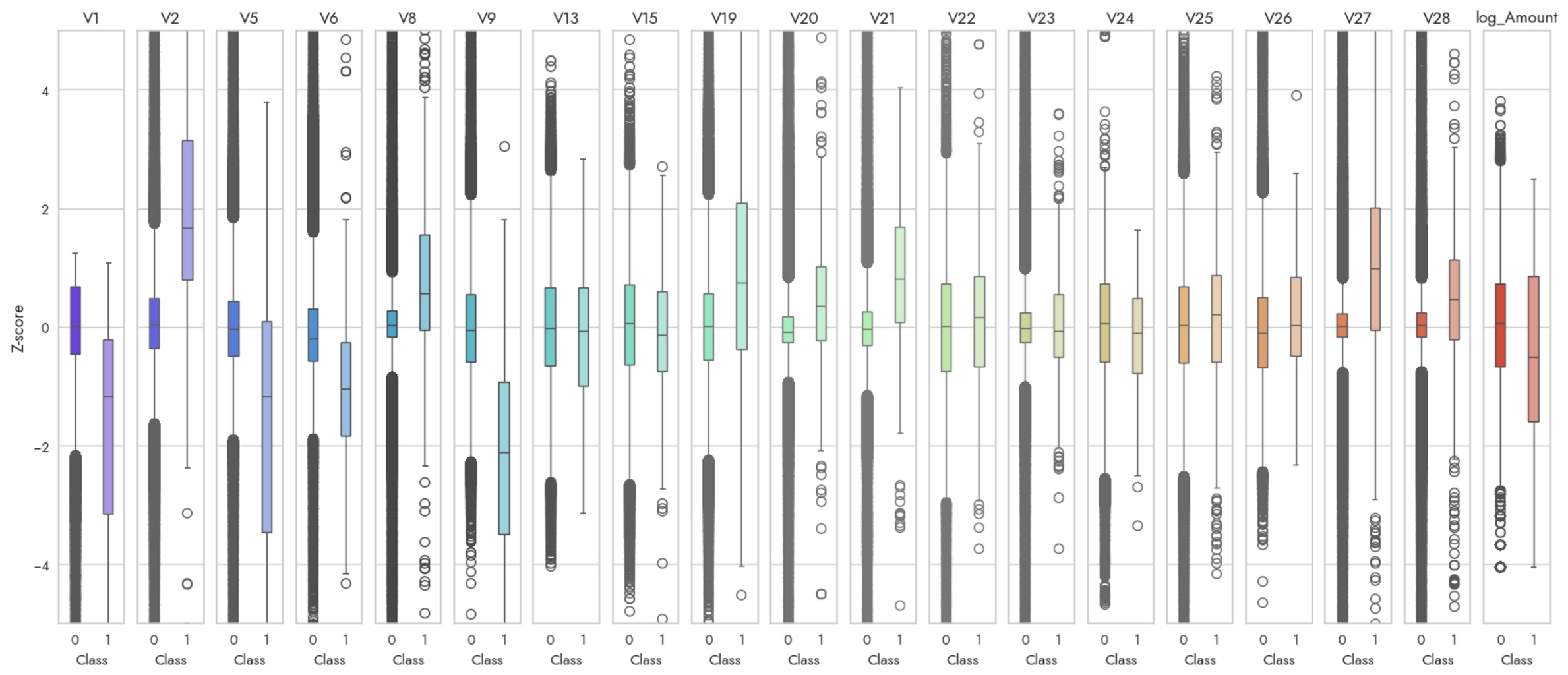
There’s certainly something noteworthy about the distinct distributions for V1, V2, V5, and V9 that is also compelling. Indeed, re-running SelectKBest with k=15 instead, we add on V1, V2, V5, V6 (perhaps less apparent), and V9. This proves these features are also worth including in a first pass.

So now that we have some leads, how can we determine which of these 16 features is really worth keeping for our final model? A classical technique like lasso could be used to force coefficients of less important features towards zero. If we think our data might not have a linear relationship between the features and response, then we might use something like a Random Forest (RF). sklearn's SelectFromModel can be used in conjunction with a RF to perform feature selection using the RF's impurity-based feature importances. Another method could be to recursively eliminate features (RFE) using cross validation. Again sklearn provides a helpful RFECV function to do just that. From SelectFromModel we get ['V4', 'V7', 'V9', 'V10', 'V11', 'V12', 'V14', 'V16', 'V17', 'V18'], and these are also the exact same features that RFECV picks. We'll hang on to Hours as well, since it seemed relatively useful from our distribution plots earlier. As a sanity check, we can do a cross validation run of a RF with all features vs. our selected ones to see if we suffer a significant performance drop. We find that including all features returns an F1 of 0.851 with a SD of 0.021, compared to an F1 score of 0.845 with a SD of 0.017 for our selected features. So there's not a huge performance tradeoff while we massively simplify from 30 features to just 10.

Modeling

Our subset of features thrown into a cross-validated Random Forest model seems to get pretty strong performance with an F1 score of 0.85. Let's visualize the model's predicted probabilities on our most important features (V17, V14, V12) according to SelectFromModel.

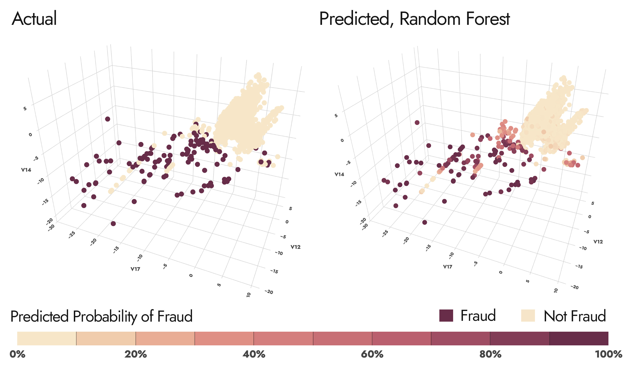
This is pretty interesting, because we can see a very dense cluster of "not fraud" to the right of each graph, and a sparser scattered cluster of fraud to the left of each graph, with the exception of a few "lines" of not-fraud interspersed. This gave me the idea that this problem can be framed as two sub-problems. One is to identify which cluster a transaction belongs to (a "first pass" to see if there's anything suspicious about the transaction). If it's the right cluster, we can be reasonably confident it's okay. If it's the left cluster, we have some further modeling to do (and a RF seems to capture the non-linear relationship here well). For the first subproblem, let's give a classic Logistic Regression a shot.

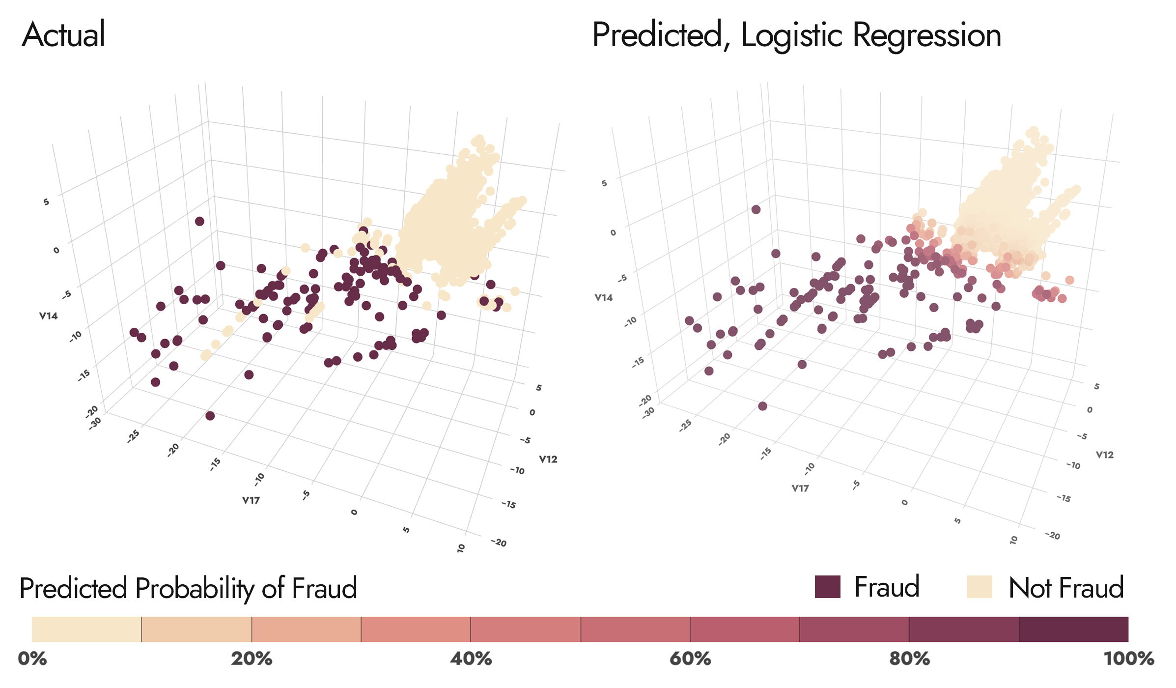
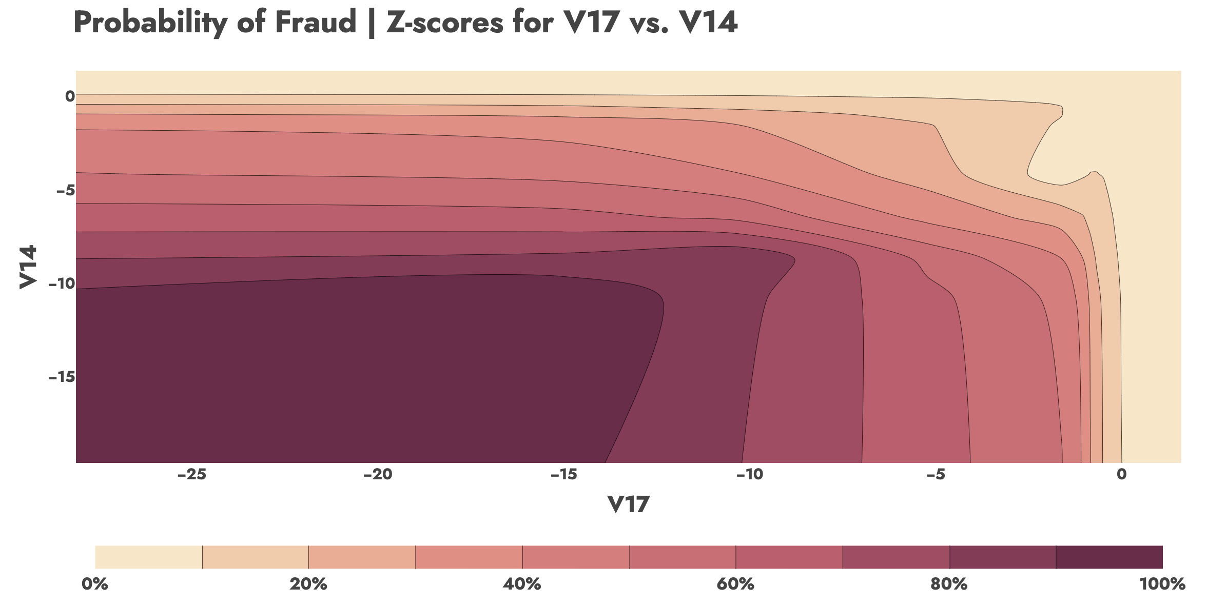
Logistic Regression gives us an F1 score of 0.76 with just those three features, achieving a 0.745 Precision and 0.770 Recall. Really impressive! Logistic Regression is of course easily interpretable. In the contour chart below, we can fix V12 at its median value and observe how the decision boundaries of fraud probabilities between V14 and V17 change with their Z-scores.

I chose a two stage approach. I trained and hyperparameter tuned a RF with K-fold (K=5) cross-validation on a subset of the original training data. The subset was all transactions where the Logistic Regression predicted a >1% probability of fraud.

I ultimately chose to go with a Logistic Regression for a first pass with a more conservative decision threshold of 0.001. If the transaction was below this threshold, it was classified as "not fraud" since the Logistic Regression model estimated that the probability of fraud was just 0.1%. If the transaction was above this threshold, it was given to a RF for further evaluation. Of ~85k transactions in the holdout test set, ~45k were determined to not be fraud, and only 4 actually were. That is a 0.01% false negative rate while achieving a constant runtime 50% reduction in the size of the problem!

LogReg	Actual 1	Actual 0
Predicted 1	0	0
Predicted 0	4	44681

The second stage was feeding all the transactions with a >0.1% probability of fraud to the RF. The second stage achieved an F1 score of 0.863, with a Recall of 0.785 and a Precision of 0.958. Out of 40k remaining transactions to classify, all but 36 were correctly classified. There were 31 false negatives and only 5 false positives.

RF	Actual 1	Actual 0
Predicted 1	113	5
Predicted 0	31	40609

The combined confusion matrix of the two stages is:

Combined	Actual 1	Actual 0
Predicted 1	113	5
Predicted 0	35	85290

The combined model achieves an F1-score of 0.85, combined recall of 0.76, and combined precision of 0.96. Note that this is very often identical to the result as ONLY using RF. The Logistic Regression step does not meaningfully change our model performance on precision and recall, but rather offers a speedup and transparent visibility into many of the non-fraud classifications. I believe that it is going to be very difficult to find a model that significantly improves over these results.

Extensions

Until now we have assumed that a false negative and false positive are equally undesirable (since we use F1). This is not realistic -- a false negative (not flagging a fraud) could cost us much more than a false positive (mistakenly freezing a customer's card, which doesn't incur a cost unless that customer churns or customer service backlogs increase).

We can of course retrain our model using an F2 scoring metric (I use F1 since it makes model performance easier to compare) which will bias towards recall (fewer false negatives). We can also create a cost function that weights false negatives and false positives. Say with a ratio of 5:1 (that is to say a false negative costs around 5x as much as a false positive). Minimizing this cost function would then give us the appropriate threshold for the Random Forest, where above that predicted probability we classify fraud, and below it we classify not fraud. Since false negatives are weighted more, we should expect this threshold to be more conservative (i.e. probabilities under 50% should still be classified as fraud).

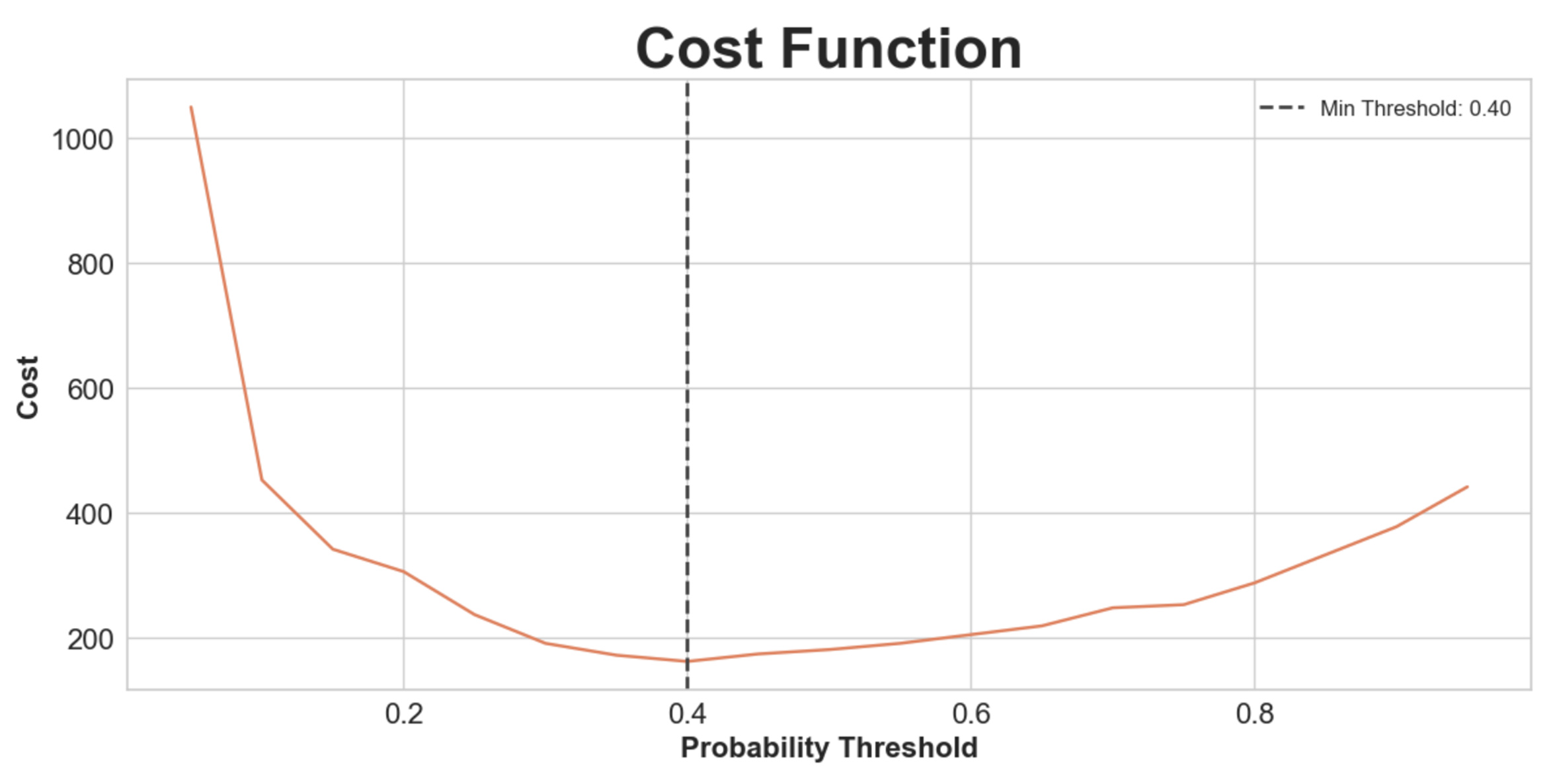
Indeed we find that 40% minimizes our cost function. At this threshold, our confusion matrix is outlined below. We trade 6 fewer false negatives for 11 more false positives, which according to our cost function is worth it (in fact it would take 30 false positives before it's not worth it).

Combined	Actual 1	Actual 0
Predicted 1	119	16
Predicted 0	29	85279

So we get a slightly worse F1-score of 0.84 and worse Precision of 0.88, but we minimize our hypothetical cost function and improve Recall to 0.80. The goal here is not to maximize a specific out-of-the-box metric, but to parametrize the tradeoff between metrics.

Looking through Kaggle, I think there are very few examples that squeeze much better performance out of this dataset (particularly when disqualifying notebooks that have scaling/oversampling data leakage or which use accuracy as a performance metric), especially while retaining model explainability and refraining from overfitting.